| Autoguiding with the SBIG ST-7e (Please
be patient while the images load)
(Adjust brightness and contrast on your monitor for best viewing)
There are three parts
to this page.
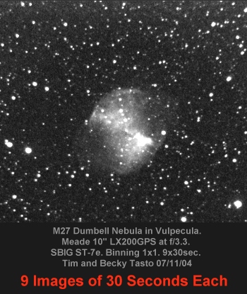
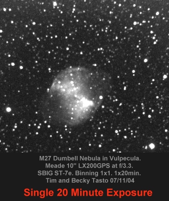
Part 1: Discusses how we got autoguiding to work with the 10" LX200GPS and SBIG ST-7e. Part 2: Discusses an experiment we performed to help determine if longer sub-integrations will improve our images. Part 3: Conclusions. Part 1 - Getting it Working This page shows the results of our efforts to get the SBIG ST-7e imaging device (with integrated guide chip) to autoguide a 10" LX200GPS in polar mode. We did succeed, but found that even autoguiding a telescope can be challenging, as any telescope mount is a mechanical device that can be susceptible to periodic and random errors when tracking. However, the images below demonstrate that with patience, good results are possible. Further, once autoguiding is properly set-up, it much easier and more presice than manual guiding. (Autoguiding devices are immune to many problems that can occur with manual guiding, such as trying to ignore a mosquito that is biting you, eye fatigue, mis-judged manual corrections, or cold fingers). Two things that improved our autoguiding capability are (1) Corrections were made at 0.5 second intervals instead of 10 seconds and; (2) It appears that histogram adjustments made in CCDOPS while autoguiding affects the result. By adjusting the histogram to reduce the star to just one or two bright pixels seemed to improve autoguiding significantly. We were a bit surprized by this because we thought that the histogram adjustment only affected what *we* see, and not what the autoguider sees. Still not sure about this one but as long as it works, we'll do it! The maximum error observed in CCDOPS during these 10 minute integrations was about + or - one pixel. Not perfect, but not too bad either. The stars are not perfectly round. A Meade f/3.3 focal reducer was used without one of the spacers to obtain an effective focal ratio of approximately f/5. Some of the minor distortions in the image are due in part to optical effects resulting from the use of the focal reducer. The ultimate solution probably lies in installing an Adaptive Optics device on the system. But, see Part 2 below! 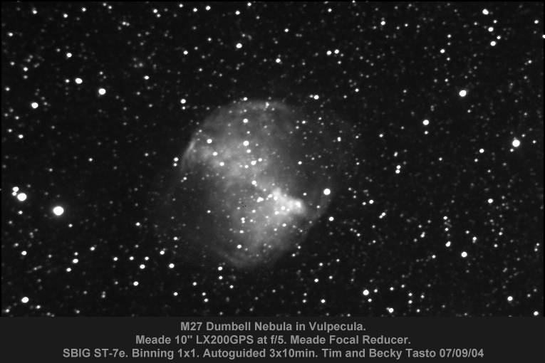 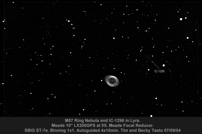 By adjusting brightness and contrast on your monitor you may be able to just barely see the faint galaxy IC-1296 in the image of M57 above. Part 2 - Which is Which? This part shows two images of M27 for comparison of imaging techniques. Both images were taken on the same night under similar conditions and with the same equipment (SBIG ST-7e and 10" LX200GPS). Both images were taken using a Meade F/3.3 focal reducer. The primary difference between the images is that one is a stack of nine 30-second exposures (9x30 seconds), while the other is a single 20-minute exposure (1x20 minutes) that was autoguided. Post-processing involved simple image calibration using a dark frame, flat field and sharpen in CCDOPS. Minimal processing was used to retain as much "raw" data as possible. Can you tell them apart?
The image on the right is slightly "smoother" than the one on the left. At first, we were surprized by this result. We expected a larger visual difference in the SNR of the images. Upon further reflection, however, the result actually makes sense. An explanation is discussed below. First, it should be noted that if one is shooting for very long (e.g. 5-hours) of total exposure, then the differences between the images would likely become much more significant. I would expect that the readout noise from trying to stack numerous 30-second sub-integrations to get 5-hours total exposure would be significantly greater than stacking a few 30-minute sub-integrations. Now, in regard to the results of our specific experiment: Relative improvement of Signal to Noise Ratios (SNR) in images based on total integration time can be estimated as follows: SNR Improvement = SQRT (20 minutes / 4.5 minutes) = SQRT(4.4) = 2.1 This is not a huge difference, and the visual impact is also minimal. However, if the total exposure of an image is 5-hours, then we are up to 300 minutes of total exposure and: SNR Improvement = SQRT (300 minutes / 4.5 minutes) = SQRT(66.7) = 8.2 Now the difference is significant and should result in notable visual impact compared to the 4.5 minute exposure. In general, increasing the exposure by a factor of ten will improve SNR by a factor of SQRT(10) = 3.2. Part 3 - Conclusions: 1) The fact that we did not see a huge difference in SNR in our experiment is because the difference in total exposure time between the two images is probably not large enough. 3) For "normal" or short total exposures (e.g. < 2-hours), stacking short sub-integrations will yield reasonable results. Noise tends to follow 1 / SQRT (N), where N is the number of sub-integrations. So stacking more sub-integrations will indeed help reduce overall noise in the final image (but will not be superior to taking a single integration due to noise that is encountered for every sub-integration that is read-out). Return to Deep Space Imaging and Astrophotography Main Page All images copyright (c) Tim Tasto and Becky Tasto SBIG, Autoguide, Autoguiding, ST-7e
|